Food-SSAFE Operation Manual (Model 971)

1Introduction

Version 1.0, 01 January 2012. Operation Manual for the Food-SSAFE Spectrum / Sample Analysis and Food Examination Kit, run through the Food-SSAFE software on the connected Model 970 multichannel analyzer (MCA).

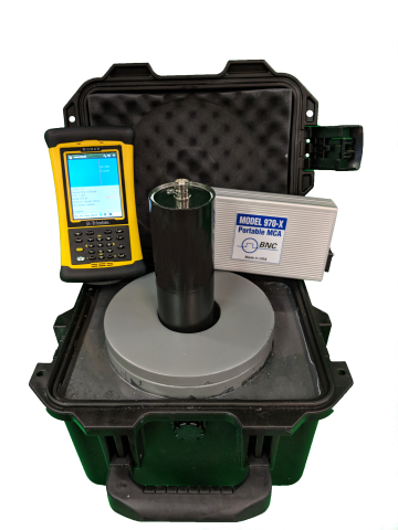
Thank you for purchasing the Spectrum / Sample Analysis and Food Examination Kit (FOOD-SSAFE). This system has been assembled to provide everything needed to quantitatively assay soil, water, air, and wipe samples for gamma-emitting radionuclides.

The FOOD-SSAFE is shipped fully calibrated to quantify water and soil samples using a 500 mL Marinelli geometry, as well as wipes and air samples using a 2″ (~3 cm) filter.

2Contents of Food-SSAFE Kit

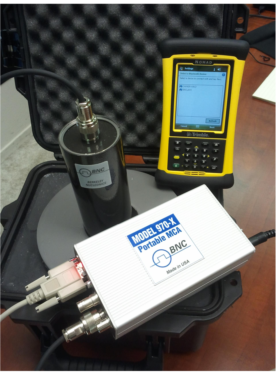
• MODEL 970 Multi-Channel Analyzer
• 2″ by 2″ NaI(Tl) gamma detector
• Detector Cable (“C” to “C” connectors)
• Trimble Nomad 900 LE with barcode scanner and serial boot, pre-loaded with Food-SSAFE software
• Charger / Power supply for MODEL 970
• Charger / Power supply for Nomad
• Serial cable
• USB Cable
• Nomad accessory pack (styli, software CD, screen protector, etc.)
• K-40 check source in Marinelli beaker
• 10 Marinelli beakers
• Spacer (0.5″ foam disk)
• Scale
• Sieve with 1/8″ screen
• Hand Shovel
• Portable Lead Shield
• Radiation Alert Inspector with Wipe Test Plate
• Lead Shield Case

Note: The MODEL 970 hardware is unmodified and can still be used with the standard MODEL 970 MCA software for Windows PCs and Windows Mobile hand-held devices.

3General Operation: Setup

1. Preliminary

a. Make sure the batteries are charged for both the MODEL 970 and the Nomad, unless you will be operating off of AC power.

b. Do your best to make sure the detector has been acclimated to the environmental conditions, such as temperature and background, by allowing the probe to sit in the area that you will be conducting your samples for a period of 10 minutes or more.

2. Putting It Together

a. While the MODEL 970 is not powered, use the “C” to “C” detector cable to connect the detector to Input 1 on the MODEL 970. NEVER connect or disconnect a detector while the MODEL 970 is powered on!

b. Use the serial cable to connect the MODEL 970 to the Nomad.

c. If you are not planning to run the MODEL 970 using the rechargeable batteries, insert the power connectors and plug into AC power.

d. Power on the MODEL 970. Allow it to run for a few minutes in order to warm up.

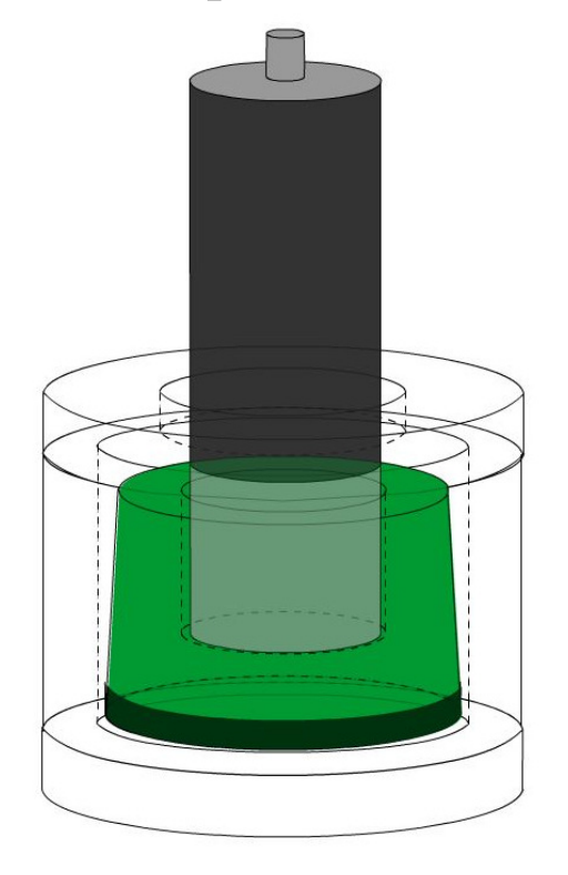
e. Place the K-40 Marinelli standard in the shield. Marinelli containers are placed with the lid on the bottom and the cavity on the top. Place the spacer into the cavity in the Marinelli.

f. Put the lid on the shield. Place the detector through the hole in the top of the shield.

3. Initial Connection

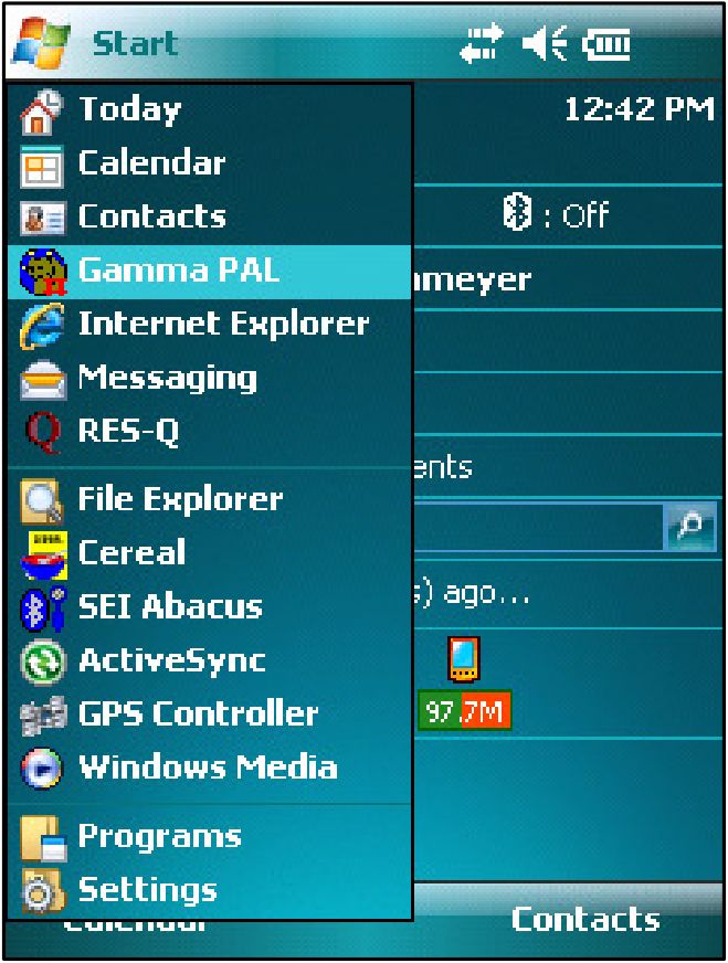
a. Power on the Nomad. Navigate to the home screen (if needed) and tap the Start icon, and then tap the Food-SSAFE icon.

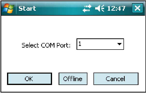
b. On the Connection screen confirm that COM 1 is indicated and tap OK to continue. The screen will close and after a few moments a message will pop up showing the serial number of the connected MODEL 970. Acknowledge that message by tapping OK.

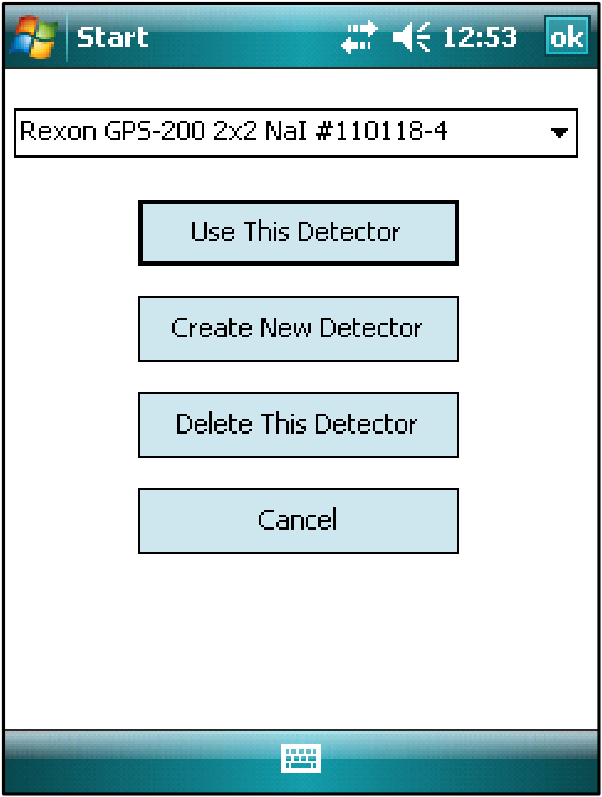
c. Next the Detector Selection screen will be shown. Confirm that your detector serial number is shown and tap Use This Detector to continue.

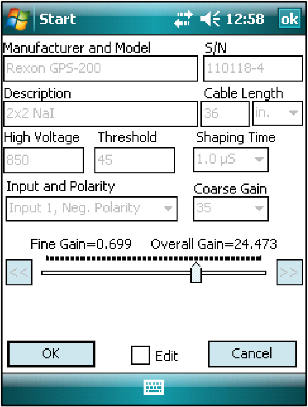
d. The Detector Settings screen is displayed. Tap the OK button to continue. This screen will disappear for a few moments (about four seconds) while the application transmits those settings to the MODEL 970.

e. When the Main Screen is displayed the system is ready to operate.

4Gain Stabilization and Source Check

Note: Prior to measuring samples the software requires that a gain stabilization and source check be performed. It is possible to bypass or shorten these requirements by using the manual gain stabilization function instead of the automatic gain stabilization, although bypassing the automatic gain stabilization is not recommended (discussed later in the section Bypassing Startup Requirements). For this quick start guide only the automatic functions are discussed.

It is assumed that the K-40 Marinelli standard and detector are set up as described above in step 2. Since the same source is used for both gain stabilization and source checking it is possible to perform both with a single acquisition.

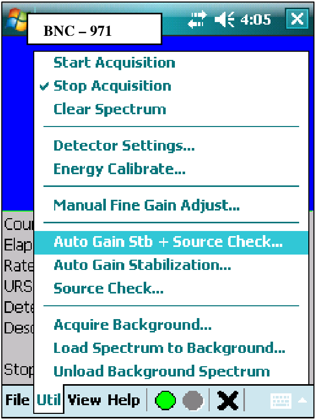
a. From the Util menu, select Auto Gain Stb + Src Check… A message pops up asking you to confirm that the K-40 source is on the detector. Tap OK to continue.

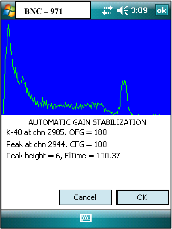
b. The Automatic Gain Stabilization screen will be displayed. The software will collect a spectrum until a sufficient number of counts exist to determine a statistically reliable peak center. If not within a few channels of the expected location the fine gain will be adjusted in the appropriate direction and an additional count started.

Displayed information includes the channel at which the K-40 peak is expected; the original fine gain setting; the centroid of the current peak; the current fine gain setting; the current peak height at the centroid; and the time elapsed in the current spectrum.

c. Once the software is satisfied with the location of the peak, the Automatic Gain Stabilization window will close and the K-40 source check will continue on the main screen. Allow this acquisition to continue until complete.

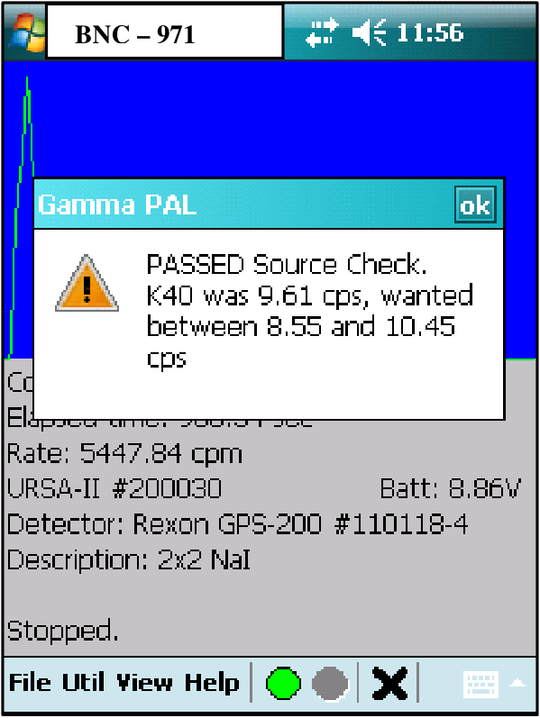
d. When the source check is complete a message will display showing the observed count rate for the source, the limits (±10% by default), and whether the test was passed or not. Acknowledge the message by tapping OK and the system is ready to begin analyzing samples.

e. Use File | Save Spectrum to save a copy of the spectrum if desired.

5Taking a Background Measurement

a. Remove the detector from the shield, take the lid off the shield, remove the K-40 standard, and recover the Marinelli spacer from the standard.

b. Place the spacer into a clean, empty Marinelli. Put the Marinelli into the shield, replace the cover, and put the detector through the hole in the shield.

c. From the Util menu select Acquire Background…

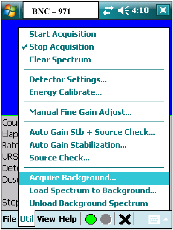
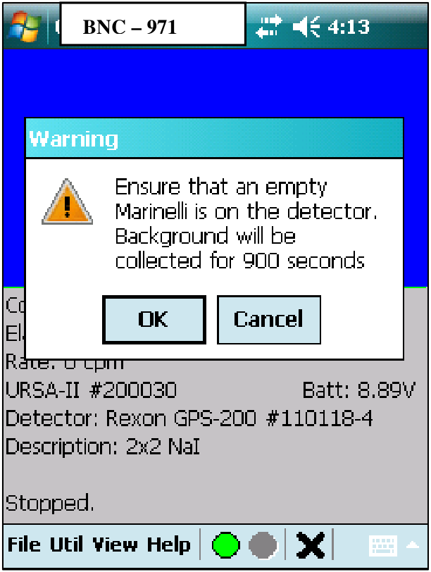
d. A message will pop up asking you to confirm that an empty Marinelli is on the detector and stating how long the background acquisition will be for. The default time is 900 seconds.

6Analyzing a Sample

a. Remove the detector from the shield, take the lid off the shield, remove the empty Marinelli, and recover the Marinelli spacer from the standard.

b. Place the sample to be analyzed in the shield. (If you are analyzing an air sample filter or wipe sample, insert the wipe/filter spacer first and put the sample into that.)

c. Place the Marinelli spacer into the cavity in the Marinelli.

d. Put the lid on the shield. Stick the detector through the hole and seat it on the spacer.

e. If a spectrum is currently displayed, tap the “X” button along the bottom of the screen (or use Util | Clear Spectrum) to clear it. If the spectrum hasn’t been saved a warning to that effect will be displayed, giving you the opportunity to save it if desired.

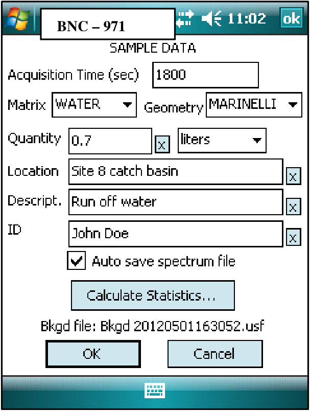
f. Tap the green circle “GO” icon (or Util | Start Acquisition) along the bottom of the screen to begin analyzing a sample. The Sample Data screen will be displayed. Enter the acquisition time desired (default is 900 seconds or 15 minutes).

Select the appropriate sample matrix (SOIL, WATER, or FILTER) and the relevant sample geometry (MARINELLI or DISK).

Note: The Food-SSAFE comes calibrated for water and soil in a (nominal 500 mL) Marinelli geometry plus a 2″ filter in a disk geometry.

Enter the quantity of the sample and units (e.g., 0.7 liters, 0.540 kg, etc.). Three more fields are available: Location, Description, and ID. These can be used for whatever purpose makes sense to your program or the fields can be left blank. Check the box next to Auto save spectrum file to have the spectrum automatically saved at the end of the acquisition.

If a background file has been loaded, the Calculate Statistics button can be pressed to determine the MDA (total Bq) and LLD (activity/quantity, e.g. Bq/liter or Bq/Kg) to ensure that the sample analysis can meet the statistical target.

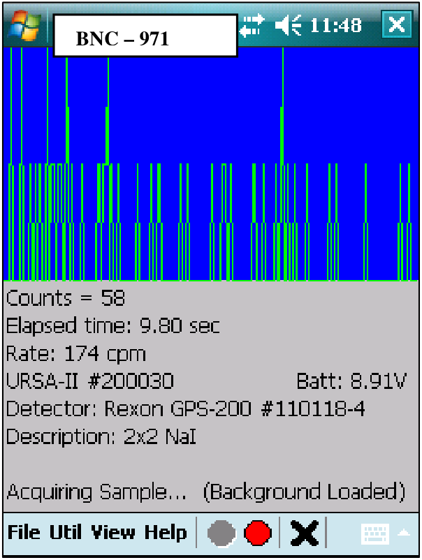
g. Tap the OK button to begin the acquisition. The main screen will be displayed with the data updated approximately each second.

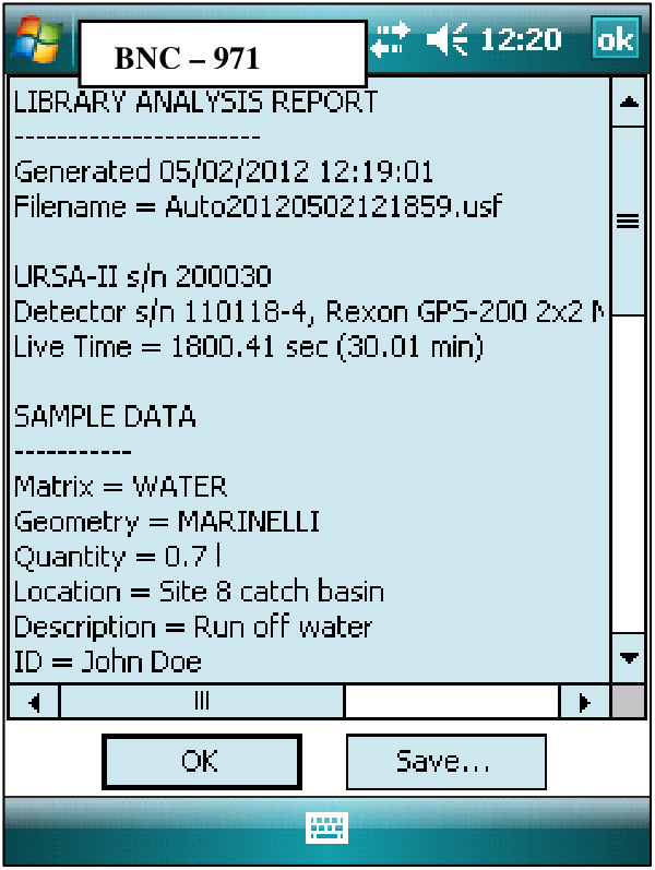
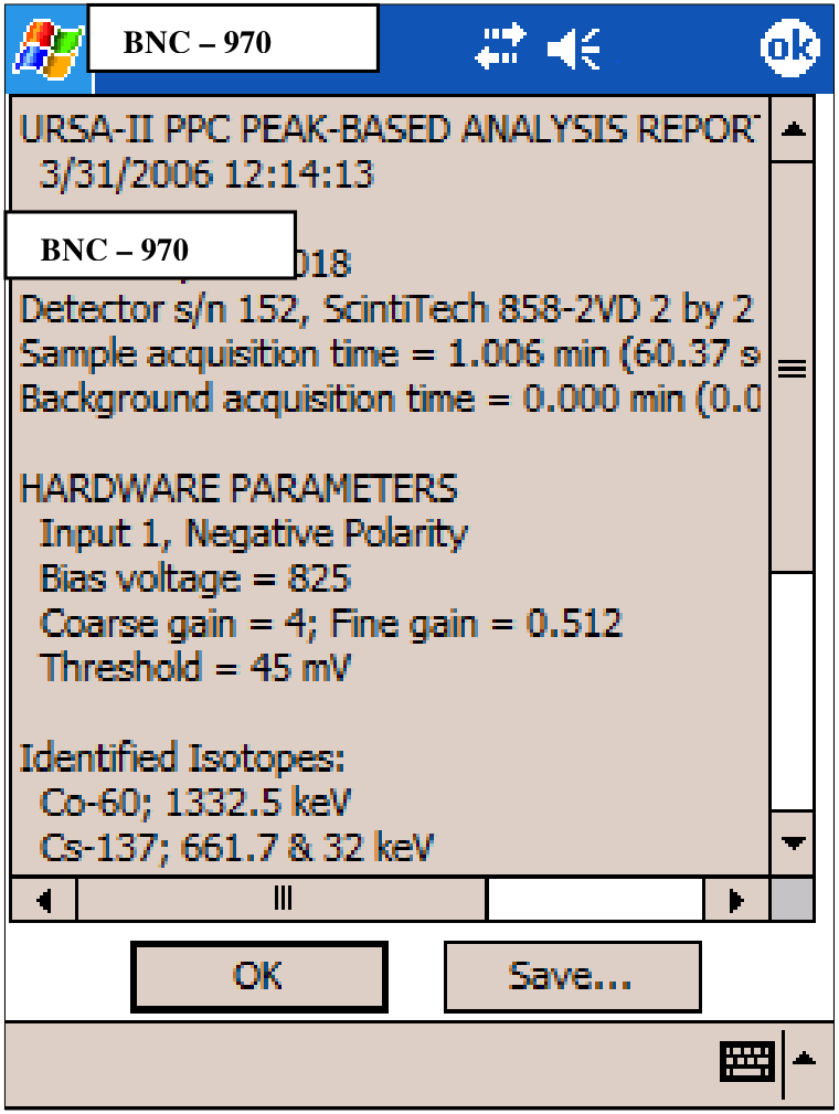
h. Once the acquisition time has been met (or if the acquisition is terminated by either tapping the “STOP” icon, or using Util | Stop Acquisition, along the bottom of the screen), an analysis of the spectrum will be performed and the report screen will be opened. Use the scroll bars to see the complete report. Tap the Save… button to save to a text file. Reports are not saved unless explicitly directed.

7Basic Functions of the Main Screen

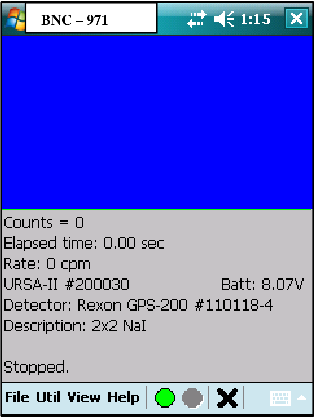
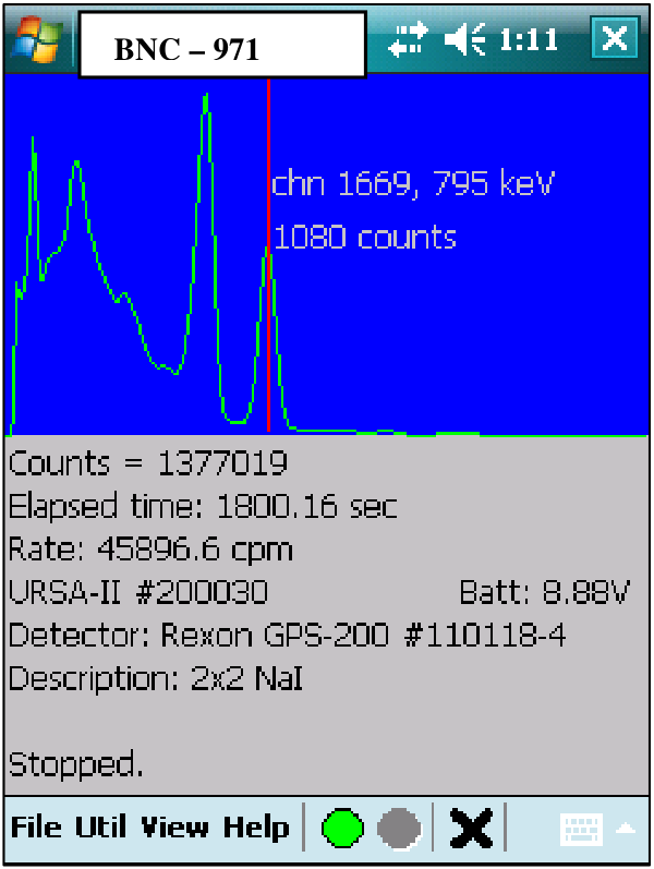
The Main Screen is divided into three sections. The top section (colored blue by default) is the Spectrum Display.

a. Colors for the background and spectrum trace (as well as for other items) can be changed using View | Preferences.

b. Tapping the Spectrum Display will cause a line to be displayed at the tapped location. The channel number and number of counts in that channel will be displayed. If an energy calibration has been performed the energy (in keV) will also be displayed. Tapping in the area beneath the Spectrum Display will hide the line. Alternately, use View | View Preferences to set a timed line display where the line will be hidden after a set number of seconds.

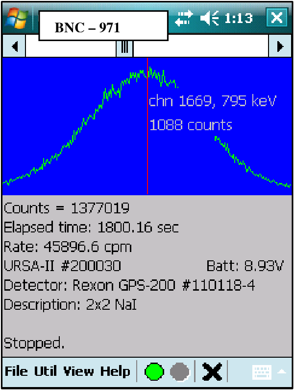
c. A MODEL 970 spectrum (4096 channels) contains more data than can be displayed, as the PPC screen is only 240 pixels wide. This means that in normal (Full Screen) mode, each screen pixel represents the sum of about 17 channels. To view a section of the spectrum in the greatest detail (one channel per pixel) select View | Zoom. If the Spectrum Display has been tapped the zoomed display will be centered on the tapped channel. When zoomed, using the scroll bar on the top of the zoomed display can move the section being viewed. The display will automatically scale to the channel with the greatest number of counts in the displayed region. Return to the normal view by tapping View | Zoom again to uncheck the item.

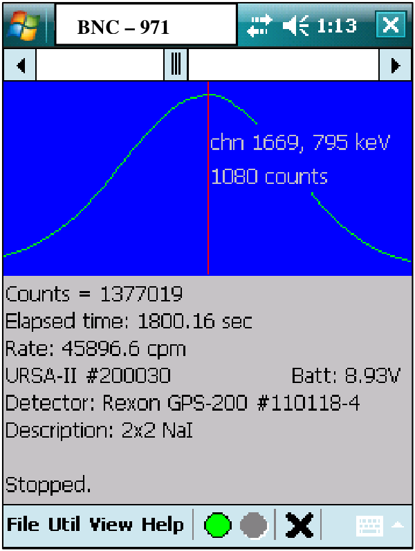
d. The spectrum display can also be smoothed by selecting View | Smoothed Spectrum. Select View | Smoothed Spectrum again to uncheck the item and go back to the raw data display.

e. The lower area (gray background by default) contains information about the current MODEL 970 and detector as well as sample acquisition information. The top line contains the total number of counts in the entire spectrum. The second line is the total elapsed spectrum acquisition time. The third line is the count rate (in cpm) from about the most recent 20 seconds of the acquisition. The fourth, fifth, and sixth lines contain the MODEL 970 serial number, the detector manufacturer, model, serial number, and the detector description. The final line contains relevant information on acquisition status, background status, etc.

f. The bottom section of the screen contains the menu items and button bar. The menu items will be discussed in detail in the next section. The button bar consists of a green circle (grayed out when an acquisition is active), a red circle (grayed out when not actively acquiring a spectrum), and a black X. Tapping the green circle will begin an acquisition, the red circle stops an acquisition, and the black X will clear the spectrum (after giving a warning and opportunity to cancel the deletion).

8Menu Items: File Menu

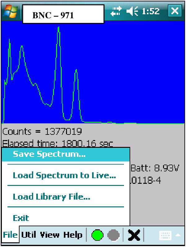
The File Menu contains functions generally related to storage and retrieval of data.

a. File | Save Spectrum allows the current spectrum to be saved to a standard “.usf” file, compatible with the MODEL 970 MCA software for the PC.

b. File | Load Spectrum to Live loads a stored spectrum into the “live” acquisition display. This is especially useful in offline mode to view and re-analyze stored spectra.

c. File | Load Library File loads a different library file to be used for analyzing samples for radioactivity.

d. File | Exit will terminate the connection and exit the application (after presenting a warning and an opportunity to cancel).

9Menu Items: Util Menu

The Util Menu contains functions generally related to calibration, detector settings, and analysis.

a. Util | Start Acquisition performs an identical function to the green circle on the button bar; it begins a sample acquisition. A checkmark will appear next to this menu item while an acquisition is active.

b. Util | Stop Acquisition performs an identical function to the red circle on the button bar; it stops a sample acquisition. A checkmark will appear next to this menu item when the MODEL 970 is not actively acquiring data.

c. Util | Clear Spectrum performs an identical function to the black X on the button bar; it will clear the spectrum (after giving a warning and an opportunity to cancel the deletion).

Detector Settings

d. Util | Detector Settings opens the Detector Settings screen. The hardware settings (HV, Threshold, Shaping Time, Input and Polarity, Coarse Gain, and Fine Gain) can be modified as needed to make the spectrum display suit your needs and purposes. The proper settings for these items were set during the initial calibration and should generally not be altered. This is because changes to these hardware settings will dramatically affect detector response, invalidating any calibrations done so far. The exception to this is the fine gain, which can be used to compensate for drift in the spectrum caused by changes in temperature, etc. Note: A separate function exists for adjusting the fine gain, covered below under Util | Fine Gain Adjust.

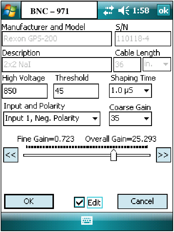
Tap the OK button to load these settings to the MODEL 970 and update the detector configuration file. Note: If the high voltage has been changed you will need to wait up to four seconds (while the MODEL 970 ramps the high voltage to the new setting) before you can begin a new acquisition.

There can only be one set of parameters for any MODEL 970/detector combination; these settings are loaded following the selection of the detector to use at program startup. You can force a single detector to have multiple settings by creating a “new” detector and changing the description, serial number, and/or manufacturer.

Tap the Cancel button to exit the screen without applying any of the changes made.

Energy Calibration

e. Util | Energy Calibrate opens the Energy Calibration dialog. The energy calibration has been performed during the factory setup and calibration. Changing any of these settings will invalidate that calibration. Instead, use the fine gain adjustment to compensate for any drift that has occurred.

In order to perform an energy calibration you should be displaying a spectrum of a known isotope. The energy calibration routine involves identifying two or more peaks and associating the channel numbers with the peak energies.

To perform an energy calibration check the Allow Edit box to enable the energy calibration controls.

Next, tap the first peak you know the energy for and a vertical line will appear. Use the right and left arrow buttons to move the line to the center of the peak. It may also be helpful to zoom the view. Enter the energy for the peak in the box marked keV:. You are not limited to whole numbers for energy values.

Use the up arrow to change the energy calibration point to 2. Un-zoom the display by checking Full and tap the second peak for which you know the energy. Use the left and right arrows to adjust the location of the line to the center of the second peak, and then enter the energy. Repeat this process for up to 12 energy calibration points.

Note: It is not strictly necessary to enter the calibration points in any order. When the energy calibration is performed the calibration points will be sorted in order of the channel values, from lowest to highest.

When all energy calibration points have been entered, tap the Do Energy Calibration button. A summary of the channels and associated energy values will be displayed in the list box. Review these for accuracy, as out-of-order values will cause strange results in later analyses.

The energy calibration is not actually stored and made active until the OK button is tapped. If the Cancel button is tapped any new values entered will be lost. The Load button can be used to load a stored spectrum into the Spectrum Display. When Allow Edit is not checked, it is still possible to use the up and down arrow buttons to scroll through the energy calibration settings.

This screen can, of course, also be used to edit any existing energy calibration. There can only be one energy calibration for any MODEL 970/detector combination. The energy calibration is loaded following the selection of the detector to use at program startup. You can force a single detector to have multiple settings by creating a new detector and changing the description. When in Offline mode, however, the energy calibration stored in the detector file (.usf) will be applied each time a new spectrum file is loaded. This does not occur when not in Offline mode.

Manual Fine Gain Adjust

f. Util | Manual Fine Gain Adjust opens the Manual Fine Gain Adjustment screen. An energy calibration must be performed before this function can be used (see below). The fine gain adjustment is intended to provide an easier way to compensate for energy drift in the detector (typically caused by temperature changes) than using the Detector Settings screen.

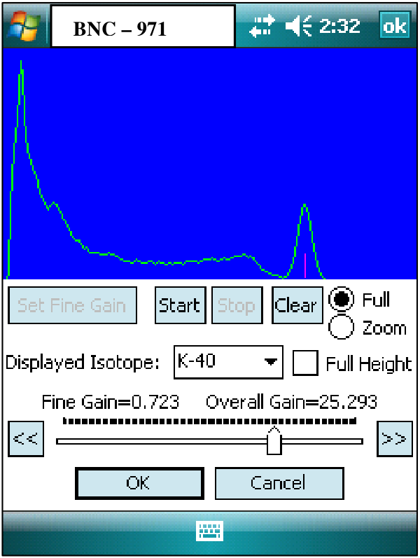
Use the Start, Stop, and Clear buttons as on the Main Screen. Acquire a spectrum of a known source and select the isotope from the dropdown list. This will cause the library energies for that isotope to be displayed on the spectrum. Checking Full Height will cause the lines to extend to the full height of the display instead of being proportional to the abundance. If the energy line does not match up with the peak, increase or decrease the fine gain control a little bit and tap the Set Fine Gain button. Then Clear the spectrum and begin another acquisition. Repeat this until the vertical line and peak line up with one another. Tap the OK button when the fine gain adjustment is complete or tap Cancel to revert to the original fine gain.

Auto Gain Stabilization and Source Check

g. Util | Auto Gain Stb + Source Check… Selecting this function begins an automated standardization routine. A message box will ask the user to confirm that the K-40 standard is in the detector. After acknowledging that the source is present a spectrum will begin accumulating. The source will be counted until the height of the K-40 peak is 8 counts, typically 2 to 3 minutes. If the location of the peak has been determined to be out of place, the fine gain will be automatically adjusted and a new acquisition started. This process repeats as needed until the K-40 peak is located at the appropriate channel.

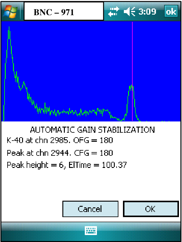
Three lines of data are displayed. The first contains the target channel for the K-40 peak and the value at which the fine gain was set when the gain stabilization was started. OFG stands for “original fine gain.” The second line shows where the K-40 peak is actually located in the current spectrum and the value at which the fine gain is currently set. The third line shows how many counts are currently under the highest point in the K-40 peak as well as the total acquisition time for the current spectrum.

Once the gain stabilization aspect is complete, the window will automatically close and the spectrum will continue accumulating as the source check.

h. Util | Auto Gain Stabilization… This function is the same as the Auto Gain Stb + Source Check function above except that when it is complete a message will be displayed to that effect and asking the user if the count of the last spectrum should be continued as the source check.

i. Util | Source Check…

j. Util | Acquire Background…

k. Util | Load Spectrum to Background… loads a spectrum file that will be subtracted (after adjusting for differences in the acquisition times) from a spectrum to be quantitatively analyzed. The background spectrum is not subtracted from the current Spectrum Display, only in analyses and during efficiency calibration.

l. Util | Unload Background Spectrum removes the background spectrum from memory so it will not be applied in subsequent analyses.

Peak Search

m. Util | Peak Search opens the Peak Search and Identification screen. A peak search is automatically performed on the current spectrum when this screen is opened. The display box shows a brief report of the results of this analysis. Double tapping on any of the “Chn” values shown in the display box will make a vertical red line appear at that particular location on the spectrum display. Found peaks are presented in order of dominance, from highest to lowest.

If too many peaks are found in the spectrum, change the sensitivity to a higher value and tap Search to re-analyze. If too few are found, decrease the sensitivity.

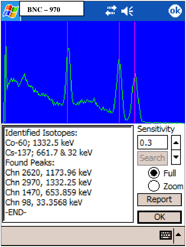
Tap Report to open the Report screen and view (and/or save) the detailed Peak Search and Identification report. Once a report has been saved, it can be synched or emailed to other recipients.

10Menu Items: View Menu

The View Menu contains functions generally related to calibration, detector settings, and analysis.

a. View | Library View brings up the Library View screen. This superimposes vertical lines over the spectrum at the locations of the library energies for any given isotope. The heights of these lines are proportional to yield unless Full is checked, in which case they extend for the length of the spectrum display.

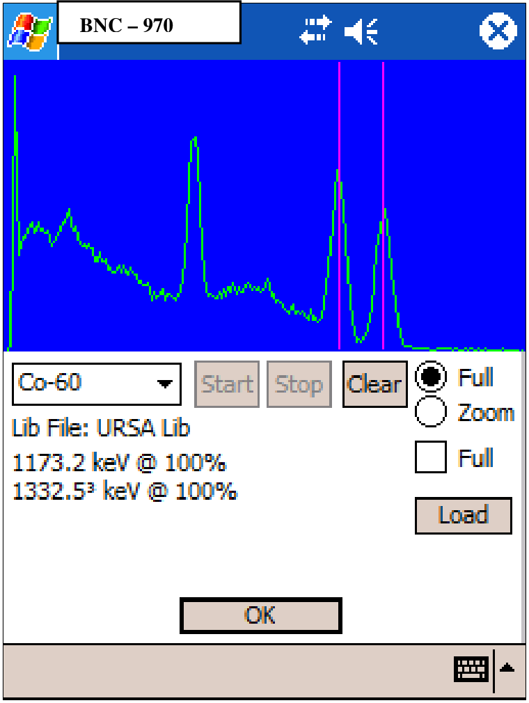
Use the Start, Stop, and Clear buttons as on the main screen. Select the isotope you would like to see from the dropdown list. The isotope data contained in the library will be displayed on the lower section of the screen. A superscript 1 indicates the primary energy; a superscript 2 indicates the secondary energy; a superscript 3 indicates that energy is both primary and secondary.

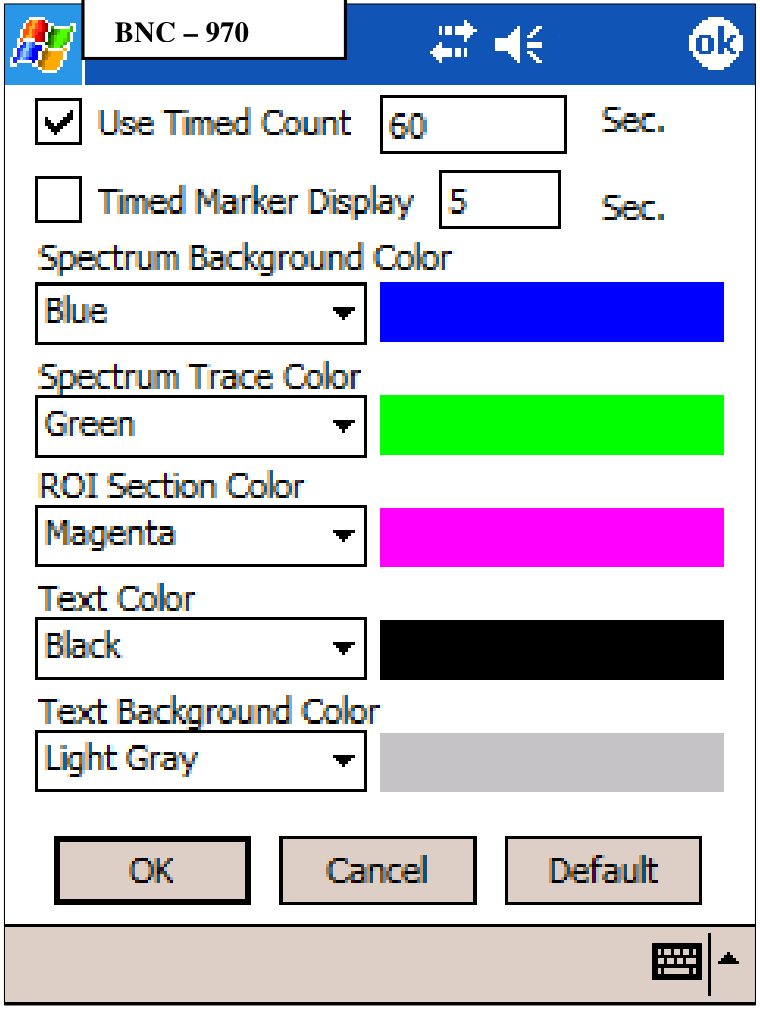
b. View | Preferences displays the Preferences screen.

If Use Timed Count is checked, acquisitions will end when the entered amount of time is met or exceeded. If unchecked, acquisitions will continue until explicitly stopped.

Timed Marker Display can be used to hide the vertical lines placed on the spectrum automatically after the entered time has elapsed. If left unchecked, markers will be displayed until an area of the screen outside of the spectrum display is tapped.

The dropdown lists are used to set colors used by MODEL 970. Use common sense when selecting colors, e.g. if the Spectrum Background Color is the same as the Spectrum Trace Color then the spectrum trace will be invisible. Use the Default button to restore the settings in place when the MODEL 970 for PPC software was started for the first time.

c. View | Full Screen is the default display for the Main Screen where the entire spectrum is compressed to fit in the width of the screen. If the display is currently zoomed, this menu item will bring it back to the unzoomed state.

d. View | Full Zoom causes the spectrum to zoom to a region 240 channels wide. If the spectrum has been tapped (and a vertical marker is displayed) then the area zoomed will be centered on this location. A slider control will appear at the top of the display allowing the zoomed portion to be moved.

11Preparation of Samples: Soil

Soil is a natural body comprised of solids (minerals and organic matter), liquid, and gases that occurs on the land surface. In order to obtain a valid result the sample needs to be prepared properly. This procedure is designed to give consistent, reproducible results for samples collected and analyzed in the field.

This procedure provides for removal of larger rocks and identifiable organic matter such as sticks, leaves, roots and vegetation.

Soils contain varying amounts of water and laboratory-based gamma spectrum analysis is performed on dried samples. Steps are included in this procedure that permit later analysis of dried samples in the laboratory if desired.

1. Using an appropriate sampling tool acquire a soil sample of 1000–1500 grams.
2. Pass the sample through the sieve provided and into a clean, dry pan or tray. Remove any identifiable organic matter from the sieved sample.
3. Label a 2-quart zip lock bag with the sample-specific information. Weigh the empty bag and record this as the tare weight of the bag. Place the sieved sample into the bag, seal the bag and weigh it. Record this weight as the gross weight of the sample. Subtracting the tare weight from the gross weight of the sample gives you the net wet weight of the sample.
4. To avoid cross contamination, clean the sieve and tray prior to processing the next sample.
5. Knead the sample gently to homogenize it.
6. Label an empty Marinelli beaker with the sample-specific information and weigh it with the cover on. Record this weight as the count tare weight.
7. Transfer the soil sample to the Marinelli ensuring that the beaker is filled completely to the top. Avoid the creation of air pockets in the sample but don’t pack the sample too tightly. Screed across the top of the Marinelli with a spatula to remove excess soil and transfer the excess back to the zip lock bag. Re-seal the bag and store the sample.
8. Replace the cover on the Marinelli, wipe any excess soil off of the exterior of the container and weigh the container. Record this weight as the gross count weight.
9. Subtract the container tare weight from the sample gross weight to obtain the net count weight of the sample. Use this weight when performing activity calculations.
10. Count the sample according to established counting protocols.

Drying Samples for Later Laboratory Counts

The advantage of drying the samples is that they can be stored indefinitely and counted at a later date. Wet samples may dry out over time giving inconsistent results as the samples lose weight because of drying. It also removes the variability of different soils having markedly different moisture levels. Also, soils may have different moisture levels at different times due to variability of rainfall and relative drought. This gives you the ability to compare data for samples taken at different times from the same site.

If you want to perform subsequent laboratory counts of dried samples follow this additional procedure:

1. After counting the field sample, transfer the sample from the Marinelli back into the labeled zip lock bag for that sample. Re-seal the zip lock bag and transport to the laboratory.
2. Weigh an oven-safe tray or bread pan. Record this as the tare weight.
3. Transfer the sample from the zip lock bag to the tray or pan and re-weigh. Record this weight as the gross wet weight.
4. Place the tray in a low temperature oven (around 250 degrees) and bake overnight.
5. Remove the pan from the oven, allow to cool and re-weigh. Record this weight as the gross dry weight.
6. Note: some soils, especially those with a lot of clay, may get very hard as a result of baking. Gently break up the soil and if necessary pass the sample through the ¼-inch sieve to break up the material.
7. Transfer the soil to a tared, labeled Marinelli ensuring that the Marinelli is filled to the top before replacing the lid. Clean any excess soil off of the Marinelli and re-weigh the sample. Record this weight as the gross dry count weight. Calculate the net dry count weight by subtracting the Marinelli tare from the gross dry count weight. Use this weight in activity calculations.
8. Calculate the % moisture of the sample using the following equation:

   

9. Back calculate the activity of the wet soil from the dry soil results using the following equation:

   

Source note. In the source PDF the right-hand side of the “Isotopic activity of wet sample (pCi/g)” equation (step 9) is blank. Only the left-hand side is printed. (verify) The full expression should be confirmed with engineering.

12Preparation of Samples: Water

Water samples consist of the chemical H₂O plus any minerals or organic matter dissolved in the matrix. Sediments and other materials suspended in the water are not generally considered to be part of the sample. If time and facilities are available the water sample should be filtered to remove as much sediment as possible. A simple coffee filter could be used for this purpose. If you are interested in counting the sediment as well, use a tared filter and count the sample using the filter protocol.

Radionuclides dissolved in water can “plate out” on the walls of the sample container over time. This can result in inaccuracies in sample analysis. If samples are to be retained for longer than 5 days they should be preserved with sufficient concentrated nitric or hydrochloric acid to bring the pH below 2.0. Generally 2 mL of concentrated nitric acid per liter of sample is adequate to achieve the target pH. Samples should be preserved after filtration. Note that preserved samples can be used for up to six months after preservation.

1. Collect the water sample in a labeled 1-liter plastic sampling bottle. If necessary, pass the sample through a tared filter to remove the sediment. Transfer the sample back into the plastic bottle. If the sample will be retained for later counting, preserve the sample with concentrated nitric or hydrochloric acid to bring the pH below 2.0.
2. Weigh a clean, labeled Marinelli beaker with the top on and record this weight as the sample tare weight.
3. Transfer the sample into the tared Marinelli beaker and ensure that the beaker is filled to the top. Place the lid on the container. Remove any excess water from the exterior of the Marinelli with a paper towel or clean cloth.
4. Weigh the sample and record the weight as the gross sample weight.
5. Subtract the container tare weight from the sample gross weight to obtain the net weight of the sample. Assume that the density of the water is 1 gm/cc and convert the weight to liters by dividing the net weight of the sample in grams by 1000. Use this volume when performing activity calculations.
6. Count the sample according to established protocols.
7. The sample can be stored in the Marinelli or transferred back to the 1000 mL bottle for storage.

13Preparation of Samples: Filters

Small samples such as wipe samples, air samples or the filtered solids from a water sample can be counted using the filter procedure. The water and soil calibration factors would give an inaccurate result when counting a sample as small as a wipe or the filtered solids from a water sample. The only sample preparation required would be for the sediment filtered from a water sample. The filter should be allowed to dry and the sample weighed prior to analysis.

1. For filtered sediment from a water sample, allow the sample to dry before analysis. The filter and sediment should be weighed and the weight recorded as the gross sample weight. Subtract the filter tare weight from the gross sample weight to give the net sample weight. Use this weight for activity calculations.
2. No sample prep is required for wipes or air filters.
3. Place the filter in a labeled zip lock sandwich bag for counting. This prevents any contaminants on the filter from being transferred to the detector and provides a convenient way to store the samples.
4. Count the sample using established protocols.

14Software License Agreement

This is a legal agreement between Paul R. Steinmeyer as well as Berkeley Nucleonics (collectively “BNC”) and you, an owner of the MODEL 970 hardware and computer program that accompanies this license agreement (the “Software”). BY INSTALLING THE SOFTWARE YOU SIGNIFY THAT YOU AGREE TO BE LEGALLY BOUND BY THE TERMS AND CONDITIONS OF THIS LICENSE AGREEMENT. These are the only terms by which RSA software products are licensed to you.

Grant of License

RSA hereby grants to you a non-exclusive, non-transferable license to use the Software according to the terms and conditions herein. Legal title to the Software and Software documentation provided under this agreement shall remain with RSA as its sole property, subject to your rights as specified in this agreement.

Description of Rights and Limitations

You may install and use this software on as many computers as you like, without restriction or limitation. You may not reverse engineer, decompile or disassemble the Software, except and only to the extent that such activity is expressly permitted by applicable law notwithstanding this limitation. You may not modify, adapt, translate, rent, lease, lend, sell, distribute or create any work deriving from the Software or any part thereof. You may use the Software and its processes for its internal purposes.

Limited Warranty

This Software is provided “as is” without warranty of any kind, to the maximum extent permitted by applicable law. RSA further disclaims all warranties, including without limitation any implied warranties of merchantability, fitness for a particular purpose, and non-infringement of patent or copyright. The entire risk arising out of the use or performance of the Software and documentation remains with you, to the maximum extent permitted by applicable law. In no event shall RSA or its suppliers be liable for any consequential, incidental, direct, indirect, special, punitive, or other damages whatsoever (including, without limitation, damages for loss of business profits, business interruption, loss of business information, or other pecuniary loss) arising out of this agreement or use of or inability to use the Software, even if RSA has been advised of the possibility of such damages.

High Risk Activities

The Software is not fault-tolerant and is not designed, manufactured or intended for use or resale as on-line control equipment in hazardous environments requiring fail-safe performance, such as in the operation of nuclear facilities, aircraft navigation or communication systems, air traffic control, direct life support machines, or weapons systems, in which the failure of the Software could lead directly to death, personal injury, or severe physical or environmental damage (“High Risk Activities”). RSA and its suppliers specifically disclaim any express or implied warranty of fitness for High Risk Activities.

Miscellaneous Provisions

By installing the Software you agree to indemnify RSA for any damages which RSA may suffer by reason of any breach of this Agreement on your part. All content accessed through the Software is the property of the applicable content owner and may be protected by applicable copyright law. This license gives you no rights to such content. No modification of this Agreement shall be valid unless made in writing and executed by RSA. Should any provision contained within any paragraph of this Agreement contravene the law of any jurisdiction in which it is to be performed, such provision shall be severed from and shall be deemed not to be a part of this Agreement, but such severance shall in no way affect any of the remaining provisions hereof or cause the same to be void.

Universal Radiation Spectrum Analyzer, FOOD-SSAFE, Food-SSAFE, URSA, MODEL 970, MODEL 970 MCA, and MODEL 970 for PPC are trademarks of Paul R. Steinmeyer. Radiation Safety Associates, Inc. and RSA are trademarks of Radiation Safety Associates, Inc. Copyright © 2000–2012, Paul R. Steinmeyer. All rights reserved.